Artificial neural networks or connectionist systems are computing systems inspired by the biological neural networks that constitute animal brains. Such systems learn tasks by considering examples, generally without task-specific programming
Basic Building Block of Artificial Neural Network:
Neuron:
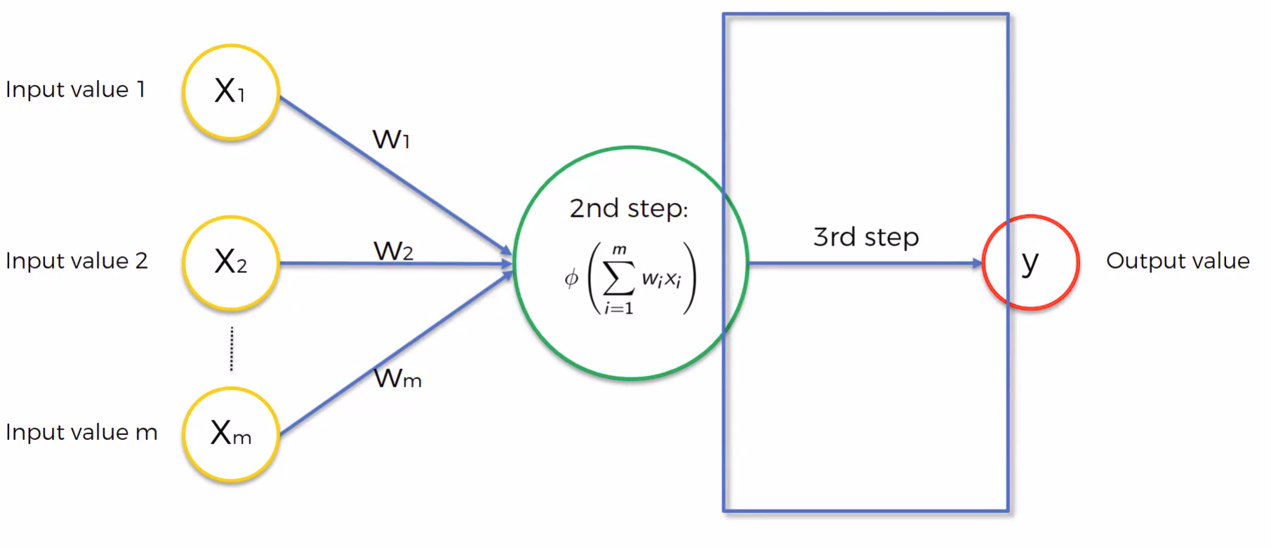
One neuron is that which takes input and pass some output. Input can be from user or from other neuron output result. Output from neuron can be the end result or can be served as a input to the other user.
Each neuron can be break into three steps.
First step it takes input, input can be one or multiple, after the input is received,
Second step is assigning weights to each input and in neural network this weights are adjusted to get the accurate output.
Third steps known as activation function takes sum of input into weight and pass the result to the output end.
Activation Function: ( Third step)
Their main purpose is to convert a input signal of a node in a A-NN to an output signal. They introduce non-linear property to our Neural Network.
Types of Activation function:
- Threshold Function:
Φ = 1 if x >= 0
0 if x <0
f(x) = Σi=1m wixi
Gives result as yes or no, can be used in place of binary result. - Sigmoid Function:
used where we try to predict probability as it is smooth curve.
Φ(x) = 1/1+e-x - Rectifier function
Φ(x) = max(x, 0) - Hyperbolic Tangent(tanh) Function:
similar to sigmoid function except it goes below zero from -1 to 1.
Φ(x) = 1-e-2x/1+e-2x
How do Neural Network work?
Each input layer has some relation with other layer may be positive or negative or combination of some input may have specific case and special result. Here comes the role of hidden layers as hidden layers tries to find out the relation between different layers along with special activation function when certain condition is met that node fires up and thus help us to handle special cases along with other case.
How do Neural Network Learns?
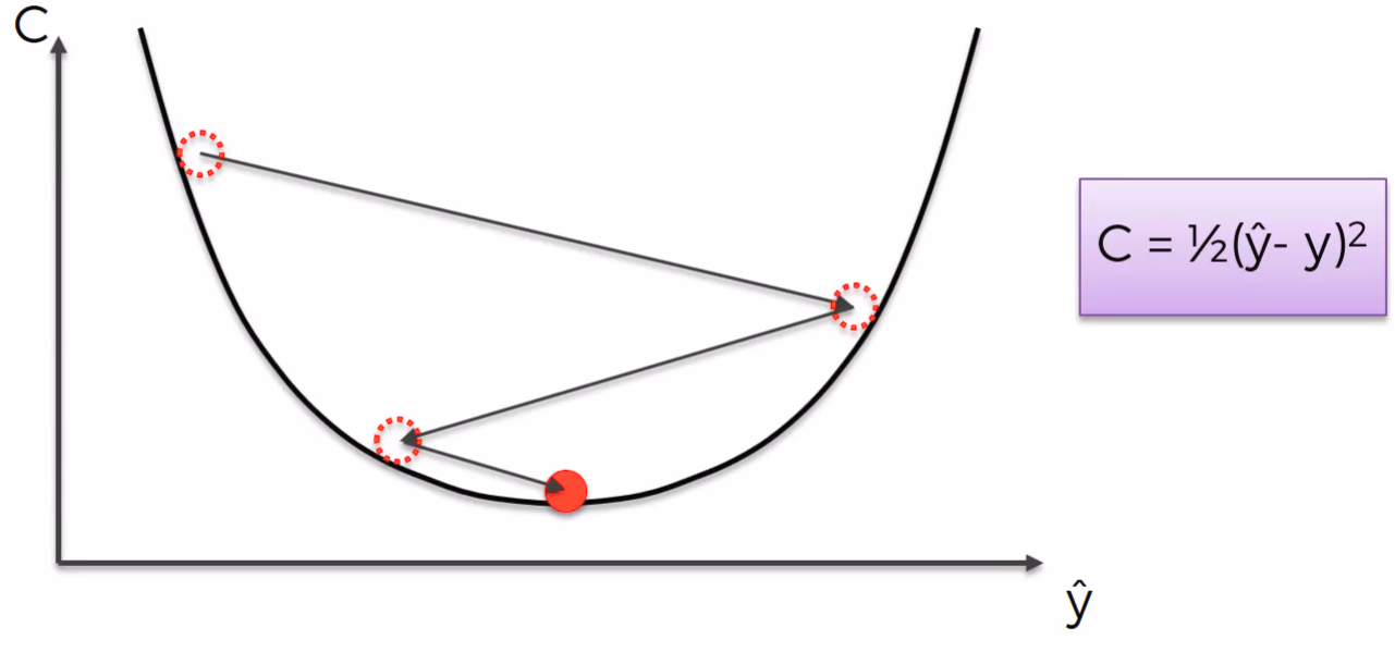
Neural Network Learns by adjusting their weight. Each row is being passed in the neural network and error is counted ie. cost function and then we adjust the weights such that cost function error is minimized and at the last we reach the optimal weights of each node. This is called Back Propagation.
Cost function = Σ 1/2 (y^-y)2
What is difference between cost function and loss function?
The loss function (or error) is for a single training example, while the cost function is over the entire training set (or mini-batch for mini-batch gradient descent)
Which Deep Learning model can classify categories which are not mutually exclusive?
You can achieve this multi-label classification by replacing the softmax with a sigmoid activation and using binary crossentropy instead of categorical crossentropy as the loss function. Then you just need one network with as many output units/neurons as you have labels.
You need to change the loss to binary crossentropy as the categorical cross entropy only gets the loss from the prediction for the positive targets. To understand this, look at the formula for the categorical crossentropy loss for one example i(class indices are j):
Li=−∑jti,jlog(pi,j)
In the normal multiclass setting, you use a softmax, so that the prediction for the correct class is directly dependent on the predictions for the other classes. If you replace the softmax by sigmoid this is no longer true, so negative examples (where ti,j=0
) are no longer used in the training! That’s why you need to change to binary crossentropy, which uses both positive and negative examples: Li=−∑jti,jlog(pi,j)−∑j(1−ti,j)log(1−pi,j)
Loss Functions:
A loss function is used to optimize the parameter values in a neural network model. Loss functions map a set of parameter values for the network onto a scalar value that indicates how well those parameter accomplish the task the network is intended to do.
Gradient Descent:
It tells us how the weights are adjusted in neural network as it is fast and efficient. It is similar to binary search but here we look for slope of cost function and cost function minima slope would be zero. so we try to try value between and keep on decreasing the range such that we get minima or slope is zero.
Stochastic Gradient Descent:
In gradient descent method we run all the rows and than we update the weight while in stochastic gradient method we keep on updating the weight after each iteration. Such that Stochastic is more memory efficient as it doesn’t need to store the every updated weight and it’ more accurate and fast. Stochastic tries to find out global minima, while if graph is not convex gradient descent fails there.
Epochs: when whole training set is passed to neural network that is one epoch.
Neural Network In Python:
Keras is library built on top of Theano and Tensorflow used for building deep neural network model.
Tip: Number of layer to be taken in hidden layer is the average of number of inputs plus no. of output node. There is no thumb rule to decide number of nodes in the hidden layers.
Activation function require to be rectifier function for hidden layer and sigmoid function for output layer.
Softmax is used for the dependent variable which have more than two categories as a output activation function.
Here the code goes…
# importing the libraries
import numpy as np
import pandas as pd
import matplotlib.pyplot as plt
# importing the dataset
dataset = pd.read_csv('Churn_Modelling.csv')
x = dataset.iloc[:, 3:13].values
y = dataset.iloc[:, 13].values
dataset.head()
# label encoding of categorical data
from sklearn.preprocessing import LabelEncoder, OneHotEncoder
labelencoder_x_1 = LabelEncoder()
x[:, 1] = labelencoder_x_1.fit_transform(x[:, 1])
labelencoder_x_2 = LabelEncoder()
x[:, 2] = labelencoder_x_2.fit_transform(x[:, 2])
onehotencoder = OneHotEncoder(categorical_features=[1])
x = onehotencoder.fit_transform(x).toarray()
# removing dummy variable trap
x = x[:, 1:]
# splitting the dataset into training and test set
from sklearn.model_selection import train_test_split
x_train, x_test, y_train, y_test = train_test_split(x, y, test_size = 0.2, random_state = 0)
# we need to apply feature scaling to reduce the time compuation time
from sklearn.preprocessing import StandardScaler
sc = StandardScaler()
x_train = sc.fit_transform(x_train)
x_test = sc.transform(x_test)
# making the ANN model
# importing the keras library and package
import keras
from keras.models import Sequential
from keras.layers import Dense
# initialising the ANN
classifier = Sequential()

# adding the input layer and hidden layer
classifier.add(Dense(6, input_shape=(11,), activation='relu'))

#adding the second hidden layer
classifier.add(Dense(6,activation='relu'))

# adding the output layer
classifier.add(Dense(1, activation='sigmoid'))

# making the prediction and evaluating the model
# categorical_cross_entropy for categorical output
classifier.compile(optimizer='adam', loss='binary_crossentropy', metrics=['accuracy'])
# fitting the ANN to the training set
classifier.fit(x_train, y_train, batch_size=10, epochs=100)
# predicting the result
y_pred = classifier.predict(x_test)
y_pred = (y_pred >0.5)
# making the confusion matrix
from sklearn.metrics import confusion_matrix
cm = confusion_matrix(y_test, y_pred)
cm
accuracy = (cm[0,0]+cm[1,1])/(cm[0,1]+cm[1,0]+cm[1,1]+cm[0,0])
accuracy*100
Next Topic: Convolutional Neural Networks
